ComfyUI Visual Stories — Part 2

Second part of the ComfyUI course material introduced in the previous post. Here the focus shifts from the individual loader modules to how they connect: the flow that runs from the Flux model through IP-Adapter and ControlNet conditioning, the two CLIPTextEncode branches (positive and negative), down to KSampler, VAE decoding, and the final saved image. The post closes with a broader reflection on how neural networks learn through repeated cycles, and an annotated diagram of the complete node chain. Previous section: ComfyUI Visual Stories — Part 1.

1. 01

   How the flow works

   Once Flux-dev is loaded, three inputs are applied to the Flux model:
   
   The first two act on the image itself: the Image Processing Adapter (IPA) and ControlNet, which modify certain internal states of the main Flux network. Following the wires between the nodes: in this pipeline, six lines leave the Flux Diffusion Model module and enter six IPA modules — one per final shot — then leave those six IPA modules and enter the six KSampler modules. These KSampler modules are the ones responsible for the Noising/Denoising process described in the introduction, controlling image generation starting from white noise (the fog discussed earlier). As for ControlNet, six lines leave the ControlNet loader and go into the module that applies ControlNet.
   
   The third input acts on the text component: it creates the conditions that activate the prompts describing the six output images. As seen in the introductory explanation, the basic mechanism is to create an image by processing a text prompt together with the other input graphic components.
   
   There is then a more elaborate mechanism, where the Flux model module is duplicated to resolve scenes in which both characters appear together. The sequence of the two modules isn't entirely clear-cut in the Flux graph's architecture, because they aren't static — they depend on the prompts (where the number of characters present in the scene is declared). The problem is therefore resolved by the internal architecture itself.
   
   We arrive at the CLIPTextEncode module, which takes as input the connection to the main Flux module, to CLIP, and to the VAE. The role of this module is to integrate Flux and CLIP and then encode them with the VAE — that is, to transform into numeric spaces the descriptive prompts for each scene (there are two per scene: clip_l + t5xxl). Note: while t5xxl is tasked with describing the scene in detail, CLIP retains its older role of also describing a negative prompt — excluding all unwanted components.
   
   Let's go over the three inputs again:

   • The main model receives FluxIPA and CLIP as input, as we saw: they coordinate image and text processing.
   • The VAE encoder transforms everything into numeric spaces so the operations can be carried out.

   At this point we reach the final steps, already described individually above: ControlNet and KSampler — the part that simulates rendering, and the part that performs Noise-Denoising. Finally, the VAE decoder brings the scene image back into plain, visible form, which can then be saved to storage.

2. 02

   A broader reflection

   One final, broader reflection. The least intuitive thing — and it wasn't, almost for anyone, even ten years ago — is that, thanks to neural networks, all the modules we've seen can be connected together and processed in cycles (many cycles) all at once. At every cycle, the weights and internal connections of the network's neurons change, and this is how the network gradually learns and transforms the information it processes — even when that information is highly heterogeneous (since it includes everything: positions, character features, colours, environments, and so on). Today's networks have become a combination of many layers (30–40 or more), where each layer is a stratum of neurons (millions of them, or more), and where the connections are guided by what's called an attention mechanism, which in short steers the flow of information. By running many cycles, the network learns. Layers + vector dimensions + attention mechanisms = parameters. When you read that a network 'has 25 billion parameters', it means it has 25 billion combinations of (layers + vector dimensions + attention mechanisms). And all of this runs hundreds or thousands of cycles — or rather, it ran them during training. This is why hundreds or thousands of GPUs are needed for pre-training, and why the costs at OpenAI, Anthropic and similar companies are so high — and why, for now, these companies operate at a loss.

3. 03

   Explanation of the main modules (second diagram)

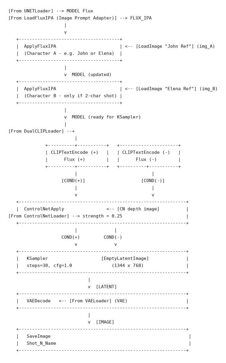
   Here is what each of the main modules shown in the flow diagram above does — the modules not already covered in the first section:

   • ApplyFluxIPA applies the IP-Adapter to the current MODEL state, injecting one character's visual identity (from their turnaround reference image) into the network's weights. It's applied once per character: first John, then Elena, when both share a scene. The second application partially overrides the first — a known limitation, mitigated by weighting the focal character higher.
   • CLIPTextEncode (+) is the positive conditioning branch: it encodes the scene prompt (composite of character-identity tokens plus shot description) into the numeric space that will guide image generation.
   • CLIPTextEncode (−) is the negative conditioning branch: it encodes what to exclude (blurry results, deformed anatomy, extra characters, and so on). At Flux's typical cfg=1.0 this has limited effect, but it's wired correctly for whenever the cfg value is raised.
   • ControlNetApply applies the depth map rendered from the 3D camera/mesh setup, at a given strength (e.g. 0.25), providing spatial and pose guidance to the model.
   • KSampler is the actual sampling engine: it performs the iterative Noising/Denoising cycle described earlier, converting random noise into the final latent image, guided by the positive/negative conditioning and by ControlNet.
   • EmptyLatentImage allocates the empty latent canvas at the target resolution (1344×768) that KSampler will progressively fill.
   • VAEDecode converts the final latent tensor into a pixel-space image, using the VAE loaded once at the top of the pipeline.
   • SaveImage writes the resulting image to disk under a per-shot filename (e.g. Shot_N_Name).

   Before running the pipeline, make sure all required custom node packs and model files are installed. The instructions page linked below lists every package, every model weight, and the files you need to provide yourself.

   ↓ Download the pipeline (JSON) → Instructions for customized modules

Previous part: ComfyUI Visual Stories — Part 1.