ComfyUI Visual Stories — Part 1

Teaching material from a short ComfyUI course aimed at filmmakers and graphic designers. A clarification first: this is not a course on video generation, but on static images that preserve identity and consistency across frames — as in comics and storyboards. The image style is hyperrealistic, meaning it aims to reproduce reality with the precision and detail of a high-resolution photograph. The course is divided into three parts: the first two are fairly theoretical in their explanation of the modules, while the third is more practical and incorporates some sections written in Python. Each component is examined in its specific role within a generative pipeline, whose JSON file is available for download. More advanced examples using this technique can be found in Comics and Storyboards.

Today, using generative AI in a controlled way — meaning not through tools that do everything in one shot, or that offer a guided-but-limited front end, or that behave as a black box — requires working the way this course describes. Every ComfyUI module/node wraps a Python function underneath (essentially 4–5 parallel neural networks calling further functions). What follows is a general overview, followed by a diagram summarising the 50+-node graph of the ComfyUI panel used in this pipeline. If parts of it aren't fully clear at first, don't worry — we'll go over everything again in the first two lessons of the course.

1. 01

   Diffusion Models: the base chain

   This course's pipeline generates images through a Diffusion Model (DM) — the generative model that marked a turning point for 'visual' AI. The main image-generating node in this pipeline is a Diffusion Model called Flux (a newer model, released in 2025 and imported into ComfyUI this year, more complex than the base architecture described below — which dates to 2022 — but fundamentally built on the same principles).
   
   The basic chain behind every Diffusion Model is: CLIP → Noise → Denoising (with cross-attention happening inside it) → VAE decoder. Let's unpack it.
   
   CLIP (you won't see it as a standalone ComfyUI node here, since it's built into the main Flux module) learns from hundreds of billions of ⟨text, image⟩ pairs how to associate an image with the text describing it. In practice this happens in geometric spaces, where both images and text are tokenised — split into fragments, which are then associated with one another. For language this is intuitive: a text splits into words, words into syllables, down to letters. For images it's less intuitive, since we're not used to fragmenting images — we can do it, but it isn't natural to find the word-fragments that match those image-fragments. In geometric spaces, though, it is possible, and this is exactly what CLIP does: it assigns a text label to an image fragment, chosen by geometric proximity (to put it in words: imagine a tree associated with every image of trees the model has learned and accepted — and this operation happens fragment by fragment). CLIP's job, ultimately, is to take every word in your prompt and associate it with the correct learned images. But this alone isn't enough to generate new images. For that, we need the other great insight behind Diffusion Models:
   
   Noising/Denoising. That is, adding noise to an image and then removing it. The metaphor here is intuitive. You're in the countryside, the sky is clear, you see a house and recognise it perfectly. Slowly, fog rises; you recognise the house less clearly, but it's still visible; the fog thickens further, until the house becomes invisible (though you retain a memory of it, even if less precise). This is the Noising process. Now think of the reverse: the fog gradually clears. Since you'd already seen the house, it takes very little — fog leaving only 10% visibility — for you to recognise it as the same house, and so on until the fog is gone entirely. At that point you're certain it's the same house, because you now see it in full clarity (this is the Denoising process). Intuitively, this is what happens mathematically so the system learns the different tokens (fragments) that make up the house — that is, so it attaches meaning to those tokens. But how does it attach meaning? By looking it up in CLIP — the function we just described, built from ⟨text, image⟩ pairs, or more precisely fragments of ⟨text, image⟩ in abstract spaces. In the end, the system — putting everything back into plain terms — has 'understood' which text fragments to associate, step by step, with the images it discovered as the fog cleared. This is what we call cross-attention in the modules below: the ability to focus on the text fragments best suited to describing the image being learned in the clear.
   
   Finally, the VAE (Variational Auto Encoder) decoder¹: skipping the technical details, the VAE decoder brings the generated image back into plain form (that is, from numerical patterns to a pixel image). We hadn't mentioned that, at the start of the Noising process, everything was first transformed into numerical patterns by a VAE encoder — to avoid overloading the explanation too early.
   
   At this point, though, comes the hardest step, I think. We've seen how the Diffusion Model manages to describe every image with text, among everything it knows. But you might ask: surely it doesn't know the exact wording of your prompt, since it's unlikely to have that exact phrase in its dataset. And indeed, it doesn't know it yet — but it manages to construct it, because a noise-prediction mechanism is also at work (predicting what the fog is covering in the image as it forms). The VAE, at the final stage of the diffusion process, stays anchored to the text just as it did during training — with the difference that here the text isn't mapped to an already-formed image, but instead guides the image being formed. This passage with/without fog drives a process of understanding and generation that is, in a fairly interesting way, similar to how the human brain works (though this parallel was only discovered afterwards).
   
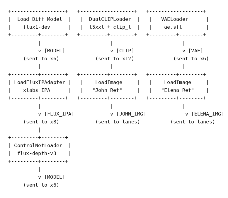
   Let's now move on to the modules that represent the neural networks — the backbone of the pipeline we've traced. The first seven boxes you see, starting from the left, are five neural networks — shown in red (Flux-dev, FluxIPAdapter, DualCLIP, VAE, ControlNet) — plus two image-loading modules for our input characters. These neural networks work together to build and structure the images so that consistency is preserved, both within each character and between characters and the environment. Let's look at them one by one.

2. 02

   Explanation of the main modules (first diagram)

   Here is what each of the seven loading modules shown in the diagram above does:

   • Flux-dev (Load) is the main neural network, the one that generates the images (a type of Diffusion Model), explained above. With appropriate bit-reduction of its numerical representations, it can run on its own on roughly 12 GB of VRAM on an RTX 3090.
   • DualCLIPLoader loads the CLIP network we've just seen. With Flux it actually loads two networks: CLIP and t5xxl. They serve roughly the same purpose — text-to-image association — but the second one supports prompts of up to 512 tokens, while CLIP is limited to around 70.
   • VAELoader loads the VAE (Variational Auto Encoder): the network that converts between the graphical pixel space and the geometric space of numerical vectors, needed to perform all the calculations. At the end of the whole chain, a VAE Decode node generates the final, plain-visible image (so there's one decoder per image).
   • LoadFluxIPAdapter loads the Image Processing Adapter network. In practice, it loads the network responsible for maintaining consistency between images across different shots, injecting visual features (i.e. characteristics of the input image) into the main Flux network to calibrate its weights. Note: at the pipeline level used in this course, this is arguably the weakest link, since it loses some consistency. In the final session of the second week I'll show how to improve it.
   • ControlNetLoader loads the ControlNet network, which adds spatial and structural conditioning to the characters' images. It isn't really a neural network but an adaptation of graphical functions proposed 3–4 years ago — such as depth maps of characters' bodies. In practice, it estimates depth and then applies it to the different poses defined in the prompts. ControlNet is independent from the IP-Adapters.
   • The two LoadImage nodes are simply loaders for the input images (the character references).

   Before running the pipeline, make sure all required custom node packs and model files are installed. The instructions page linked below lists every package, every model weight, and the files you need to provide yourself.

   ↓ Download the pipeline (JSON) → Instructions for customized modules

1. In the language of statistical mathematics for neural networks, Encoder refers to the process that transforms a pixel image into a mathematical object within a geometric space — made of points, or more precisely N-dimensional vectors. The concept of a Zip file is often used to describe it: it is, in effect, a compressed space that allows all these geometric operations to take up far less space. The Decoder is the opposite process: from the geometric space back to the plain image. ↩

Continues in the second part: ComfyUI Visual Stories — Part 2.